The block diagram of the 9th metal detector circuit setup shown in Figure 1 below, reveals two oscillators. One produces a fixed frequency of 500 kHz (F1), while the other generates a nearby frequency (F2).
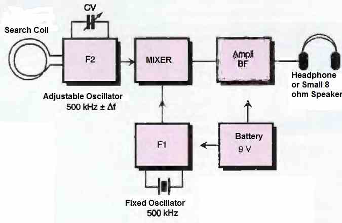
The frequency of the latter can be adjusted using a variable capacitor and modified by the presence of nearby metallic elements close to the detection coil.
After mixing, the two frequencies produce a low-frequency audible wave that allows the presence or absence of a metallic object to be detected.
How the Circuit Works
Figure 2 below introduces us to the circuit diagram of the high sensitivity metal detector. Its simple architecture is based on the utilization of two integrated circuits.
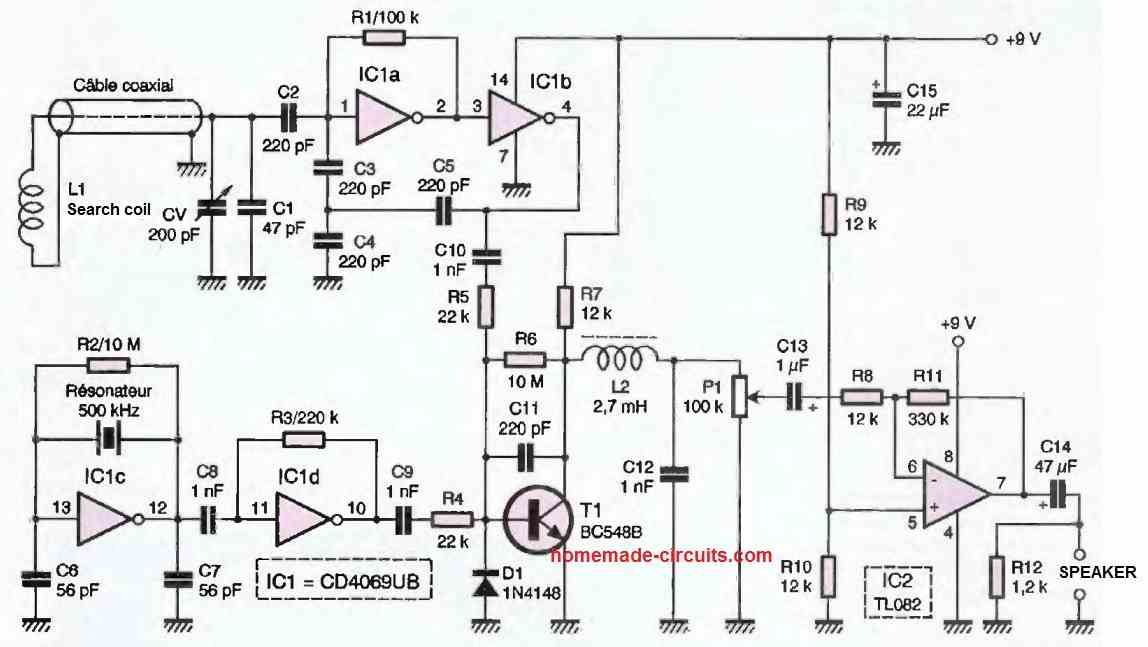
One is a CMOS, the 4069UB (unbuffered), and the other is a linear circuit, the TL082, of which only one amplifier is utilized to drive a layer or a small loudspeaker.
The fixed oscillator is realized by IC1c, mounted in the classical manner for this function. The 500 kHz resonator stabilizes the frequency.
The sinusoidal signal, available at pin 12, is fed into the input of IC1D as a buffer. At its output, we obtain a square wave signal rich in harmonics.
The variable oscillator is built around the gates IC1A and IC1B. It is a relaxation oscillator whose central frequency is determined by the LC circuit: the external coil and the variable capacitor in parallel with the series/parallel capacitors C1 and C5.
This arrangement produces a superb sinusoidal waveform of 14V peak-to-peak across the terminals of L1. The two signals F1 and F2 are applied to the base of T1 through the two networks C10/R5 and C9/R4, with values sufficient to allow for current drive.
The diode D1 prevents the signal from being aligned towards a negative value, which would no longer allow proper operation of T1.
The mixing of the two current flows F1 and F2 in the base junction of T1 results in a low-frequency voltage with a parabolic shape at the collector.
This voltage is rid of high-frequency components by the low-pass circuit L2/C12. The amplifier IC2 allows for comfortable listening after adjustment with the potentiometer P1.
Construction
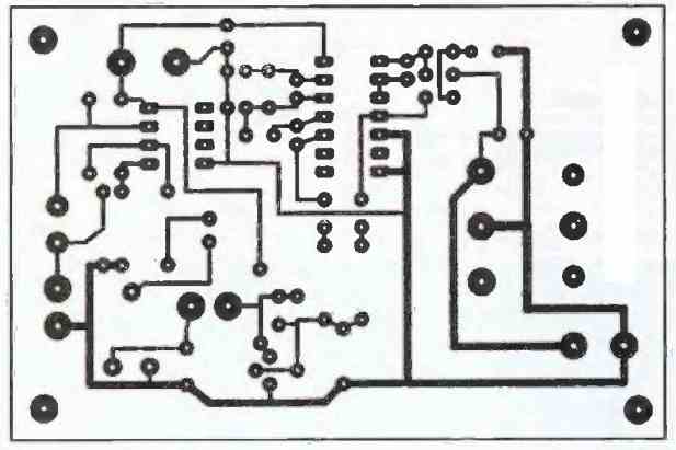
Figure 3 below shows the design of the printed circuit board at a 1:1 scale, and the next Figure 4 illustrates the component placement. There are no particular difficulties involved.
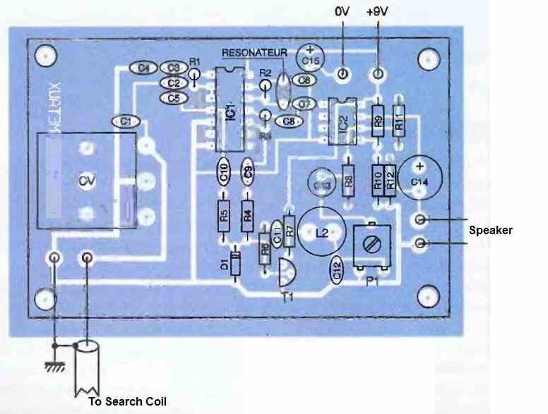
For the wiring, start with the flat resistors, the 1N4148 diode, and the integrated circuits, making sure to align them correctly. Finish by placing the standing components.
The variable capacitor is a model obtained from a longwave receiver (200 pF). However, we have also included C1 (47 uF) in parallel, which allows us to adjust the value of Cv as needed.
Note that it is also possible to parallelize the two sections of a low-value variable capacitor by bridging the free connection of Cy with the nearby trace.
The drilling of the 4 holes should be done in such a way that the components fit snugly. However, it is advisable to reinforce them with a bit of epoxy adhesive (such as Araldite), as well as the battery mounts.
How to Build the Search Coil
This highly sensitive search coil inductor was made by winding 36 turns of 0.4 mm or 0.5 mm thick enameled copper wire with a diameter of 100 mm. We used a tin can as a support.
Secure it with adhesive tape. The connecting cable is a 75-ohm coaxial cable with approximately 100 pF per meter, and it has a length of one meter as well.
We have taken into account this parallel capacitance in the calculation of the oscillator.
How to Test
Upon powering on, you will hear a more or less high-pitched whistling sound. Adjust the tone of the low-frequency signal by manipulating the variable capacitor.
It is possible to observe the effect of discrimination that can be achieved. Set the variable capacitor to produce a sound of approximately 1000 Hz.
Bringing a piece of copper close to the detector will increase the frequency. Adjust it, for the same 1000 Hz signal, on the other side of zero hertz.
This time, the proximity of the copper piece will cause the low-frequency to decrease.
The detection range varies from 1 to 10 cm depending on the mass of the metal.

Need Help? Please Leave a Comment! We value your input—Kindly keep it relevant to the above topic!