Inductors can be imagined as the opposite of capacitors. The main difference between a capacitor and an inductor is that a capacitor carries a protective dielectric between its plates, which inhibits the conduction of current across its terminals. Here it acts like an open circuit.
On the other hand the inductance of an inductor is normally (although not always) of incredibly low or minimal resistance. It essentially behaves like a closed circuit.
Capacitor Inductor Duality
There exists a unique term in electronics for this type of relationship between two parameters of a circuit or portions of a circuit. The elements of this type of pair are known as duals of one another. For example, depending on capability to conduct current, an open circuit is the dual of a closed circuit.
On the same principle, an inductor is the dual of a capacitor. The duality of inductors and capacitors is much deeper than just the natural capacity to conduct current.
In this article, we compare the working principle of inductor and capacitor of and evaluate the results with calculations and formulas.
Despite the fact that inductors normally are rarely seen in electronic circuits, since today it's mostly substituted by opamps in active filters), the other parts involved in a circuit seem to carry some quantity of inductance.
The self-inductance of the terminals of a capacitor or resistor becomes a big issue in high-frequency circuits, which explains why lead-less surface-mount resistors and capacitors are so frequently employed in such applications.
Basic Capacitor Equations
The fundamental equation for capacitors is the one with which the farad is defined:
C = Q / U [Eq.19]
where C is the capacitance in farad, Q is the charge in coulomb, and U is the pd between the plates in volts.
Through Eq. 19, we obtain an formula of the form Q = ∫ I dt + c where c is the initial charge, if available. Having identified Q, we are able to determine U from Eq. 19:
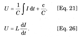
U = 1 / C ∫ I dt + c/ C [Eq.21]
An important characteristics of a capacitor can be like this, if a periodic current is applied to it (usually a current that oscillates sinusoidally), the charge on the capacitor and the voltage across it also fluctuate sinusoidally.
The charge or voltage curve is a negative cosine curve, or we can imagine it as a sine curve which lags behind the current curve by π/2 rad (90°).
The fundamental equation that defines the henry, the unit of inductance, is
L = NΦ / I [Eq.22]
With refernce to a single coil, the self-inductance in henry may be the flux relationship (the magnetic flux <1) in weber multiplied by the number of winding N, (because the magnetic flux cuts through each turn), when a unit current passes through it (I = 1 A). An even more handy definition could be extracted from Eq. 22, using Neumann’s equation. This claims that:
U = N (dΦ / dt) [Eq.23]
What this equation suggests is the fact that the e.m.f. induced within a inductor is relative to the linked rate of change of flux.
The quicker the flux varies, the higher the induced e.m.f. For instance, when the flux over the inductor or coil rises at the rate of 2 mWb s-1 , and assuming the coil has TWENTY FIVE turns, then U = 25x2 = 50V.
The path of the e.m.f. is such that it resists the variations in flux as outlined by Lenz’s Law.
This truth is oftentimes pointed out by preceding the right side of the equation with a minus sign, however so long as we believe that U is the back e.m.f., the sign could be removed.
Differentials
The term dΦ / dt in Eq. 23 indicates what I have explained as the rate of change of flux. The phrase is called the differential of Φ with respect to t, and a entire branch of arithmetic is dedicated to working with this kind of expressions. The phrase has got the form of a single number (dΦ) divided by one more quantity (dt).
Differentials are utilized to associate numerous sets of proportions: dy/dx, for instance, corelates variables x and y. When a graph is plotted using values of x across the horizontal axis and values of y across the vertical axis, dy/dx signifies how steep the slope is, or gradient, of the graph.
If U is the FET gate-source voltage, where T is the related drain current, then dI/dU signifies the quantity with which I changes for given changes in U. Alternatively we can say, dI/dU is the trans-conductance. While discussing inductors, dΦ /dt could be the rate of change of flux with time.
Calculating a differential can be regarded as the inverse procedure of integration. There isn't adequate room in this article to look into the theory of differentiation, nevertheless we will define a table of commonly used quantities along with their differentials.
Standard Differentials
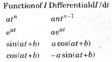
The table above works by using I and t as the factors instead of the routine x and y. So that its details are specifically pertinent to electronics.
As an example, considering that I= 3t +2, the way I deviates with respect to time can be visualized in the graph of Fig. 38. To find the rate of change of I at any moment, we estimate dI/dt, by referring to the table.
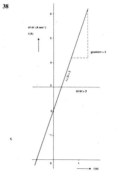
The first element in the function is 3t or, to format it as the first line of the table, 3t1 . Ifn = 1, the differential is 3t1-1 = 3t0.
Since t0 = 1, the differential is 3.
The second quantity is 2, that can be expressed as 2t0 .
This changes n = 0, and the magnitude of the differential is zero. The differential of a constant will be always zero. Getting both of these combined, we have:
dI / dt = 3
In this illustration the differential doesn't include t, that means the differential is not dependent on time.
Put simply, the slope or gradient of the curve in Fig. 38 is 3 continuously all the time. Figure 39 below displays the curve for a different function, I = 4 sin 1.5t.
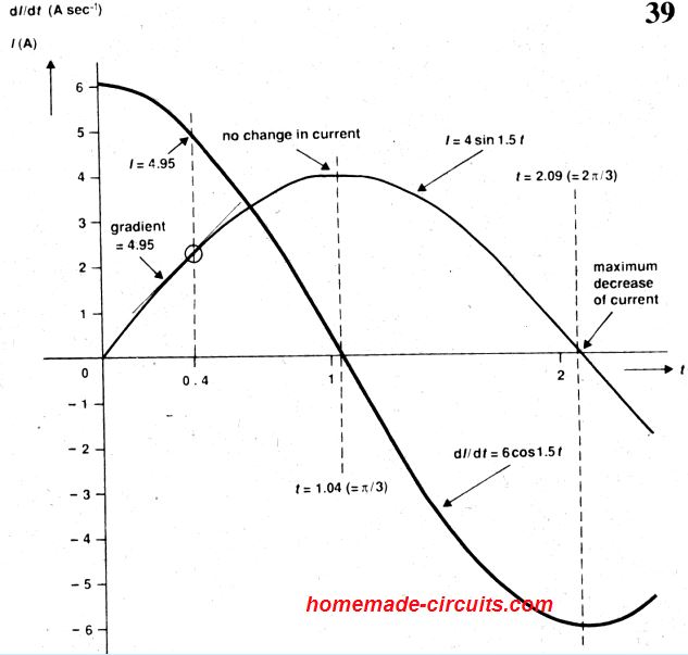
With reference to the table, α = 1.5 and b = 0 in this function. The table shows, dl/dt = 4x1.5cos1.5t = 6cos 1.5t.
This informs us the instantaneous rate of change of I. For example, at t = 0.4, dI/dt = 6cos0.6 = 4.95. This could be noticed in Fig. 39, in which the curve for 6 cos0.6t includes the value 4.95 when t = 0.4.
We can also observe that the slope of the curve 4sin1.5t is 4.95 when t = 0.4, as shown by the tangent to the curve at that point, (with respect to the different scales on the two axes).
When t = π/3, a point when the current is at its highest and constant, in this case dI/dt = 6cos(1.5xπ/3): 0, corresponding to zero change of current.
On the contrary , when t = 2π/3 and the current is switching at highest possible level from positive to negative, dI/dt = 6cosπ = -6, we see its highest negative value, exhibiting a high reduction of current.
The simple benefit of differentials is they allow us to determine rates of change for functions that are a lot more complex compared to I = 4sin 1.5t, and without having to to plot the curves.
Back to Calculations
By Reorganizing the terms in Eq 22 we get:
Φ = (L / N)I [Eq.24]
Where L and N have constant dimensions, but Φ and I may a having value with respect to time.
Differentiating the two sides of the equation with respect to time gives:
dΦ / dt = (L / N)(dI / dt) [Eq. 25]
Merging this equation with Eq.23 gives:
U = N(L/N)(dI / dt) = L (dI / dt) [Eq.26]
This is another way of expressing the henry. We can say that, a coil having self-inductance of 1 H, a change of current of 1 A s-1 generates a back e.m.f. of 1 V. Given a function which defines how a current varies with time, Eq. 26 helps us to calculate the back e.m.f. of an inductor at any instant.
Following are a few examples.
A) I= 3 (a constant current of 3 A); dl/dt = 0. You cannot find any change of current therefore the back e.m.f. is zero.
B) I = 2t (a ramp current); dI/dt = 2 A s-1. With a coil carrying L = 0.25 H, the back e.m.f. will be constant at 0.25x2 = 0.5 V.
C) I = 4sin1.5t (the sinusoidal current given in the previous illustration; dl/dt = 6cos 1.5t. Given a coil with L = 0.1 H, the instantaneous back e.m.f. is 0.6cos1.5t. The back e.m.f. follows the differential curve of Fig. 39, but with amplitude 0.6 V rather than 6 A.
Understanding "Duals"
The following two equations signify the equation of a capacitor and inductor respectively:
It helps us to determine the level of voltage produced across the component by current varying in time as per a specific funtion.
Let's evaluate the result obtained by differentiating the L and H sides of Eq.21 with respect to time.
dU / dt = (1 / C)I
As we know differentiation is the inverse of integration, differentiation of ∫I dt reverses the integration, with only I as the result.
Differentiating c/C gives zero, and rearranging the terms produces the following:
I = C.dU / dt [Eq.27]
This allows us to know the direction of the current whether it's going towards the capacitor or coming out from it, in response to a voltage varying according to a given function.
The interesting thing is that the above capacitor current equation looks similar to the voltage equation (26) of an inductor, which exhibits the capacitance, inductance duality.
Similarly, the current and potential difference (pd) or the rate of change of current and pd can be duals when applied to capacitors and inductors.
Now, let's integrate Eq.26 with respect to time to complete the equation quatret:
∫ U dt+c = LI
The integral of dI/dt is = I , we rearrange the expressions to get:
I = 1/L∫ U dt + e/L
This again looks quite similar to Eq.21, further proving the dual nature of capacitance and inductance, and their pd and current.
By now we have a set of four equations which can be used for solving capacitor and inductor related problems.
For Example Eq.27 can be applied to solve the problem as as this one:
Problem: A voltage pulse applied across a 100uF produces a curve as shown in the Fig below.
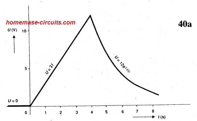
This can be defined using the following piece-wise function.
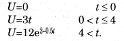
Calculate the current moving through the capacitor and plot the corresponding graphs.
Solution:
For the first stage we apply Eq.27
I = C(dU / dt) = 0
For the second instance where U may be rising with a constant rate:
I = C(dU / dt) = 3C = 300μA
This shows a constant charging current.
For the third stage when U drops in an exponential manner:
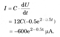
This indicates current flowing away from the capacitor in an exponential decreasing rate.
Phase Relationship
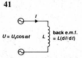
In the abobe figure, an alternating pd is applied to an inductor. This pd at any instant can be expressed as:
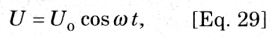
Where Uo is the peak value of the pd. If we analyze the circuit in the form of a loop, and apply Kirchhoff's voltage law in clockwise direction, we get:
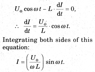
However, since the current is sinusoidal here, the terms in the bracket must have the value equal to the peak current Io, therefore we finally get:
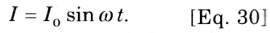
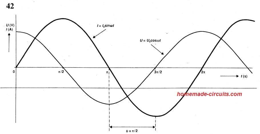
If we compare the Eq.29, and Eq.30 we find that the current I and the voltage U have the same frequency, and I lags behind U by π/2.
The resultant curves can be studies in the following diagram:
C
This shows the contrasting relationship between capacitor and inductor. For an inductor current lags the potential difference by π/2, while for a capacitor, the current leads the pd. This yet again demonstrates the dual nature of the two components.


Comments (4)
hi Mr Swagatam;
My charger for 72V battery charging (6x12V) its capacitor at the output has the value of 100V and 470uF.
I have realized that it heats. So I will raise the voltage but I am not sure on increasing the capacitance since it is an smps circuit.
So I need your comment. Thanks
Hi Suat,
Increasing the capacitance value is surely recommended and will have no negative impacts on your SMPS. So you can increase both, the voltage as well as the capacitance value…no issues.
Equation 19 is wrong.
I have corrected it now, thank you!